Animation and Creative Uses of Maths

This month's meetup in Cornwall continued the introductory series of sessions by introducing animation and seeing how mathematical functions can be used creatively.

The slides are here: [PDF].

Flip-books and Animation

Being able to move, animate, design elements adds a powerful and engaging new dimension works we create.

We started by looking at how animation is made without a computer or code - using pen and paper.

We briefly looked at this video demonstrating flip-books work.

Each page of the flip-book has an image that is slightly different from the image on the previous page. When viewed in quick succession, an illusion of movement is created.

That idea is exactly the same for digital animation. We still create animation frames, each differing from the previous one by a small change.

The following shows three frames, each with a red circle which we can think of as a ball. On the first frame the ball is near the top of the frame. In the next frame the ball is slightly lower, and in the third frame it further down.

We want to draw these frames, which could easily be from a flip-book, using code. That means thinking about the ball as a circle() shape, and its location in terms of vertical coordinates.

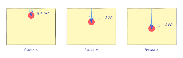
The picture shows the ball at y=50, y=100 and then at y=150. Although these are actually big jumps, the key idea is that the coordinates of the ball change with each frame.

With a flip-book, we flip each page so we seem then in quick succession. How can we do the same in code? How can we rapidly draw each frame?

We could do it manually, but p5js supports animation by providing an easy way to repeatedly call the main draw() function - the one which contains our instructions for drawing shapes and colours.

Have a look at the following simple code. We have the familiar setup() and draw() functions, with the simple.js library being initialised in setup(), and a very familiar circle() instruction in draw().

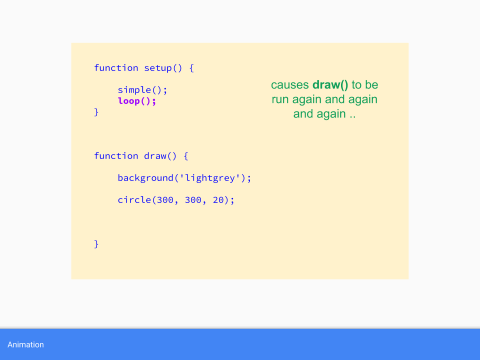
There are some new things in that code too. The loop() instruction in the setup section causes the draw() function to be called repeatedly. That's just what we need to repeatedly draw each animation frame. The background() instruction simply wipes the canvas clean with a background colour, which is just like starting a fresh new page of a flip-book.

We then turned our attention to actually drawing each frame of the animation. The following code draws a circle at (x, 300).

The important point is that x changes at every frame because it is increase by 5 inside the draw() function. Remember that draw() is called repeatedly, so x keeps increasing.

That x is initialised to 0 outside the draw() function. That means it is set before draw() is run, and is visible from draw().

Here are the results.

That worked!

Although the code, and the resulting animation, is simple - it contains all the key points fundamental to all animation:

• each frame is drawn in quick succession
• the drawing on each frame differs by a small amount
• viewed in quick succession, the frames give the illusion of movement
• incrementing/changing variables can be used to control the changing position of an object
• each new frame must be blank

We then saw how the speed of the ball could be controlled by changing the amount by which the x coordinate was incremented. Increasing it by 1 caused the ball to move slowly, and increasing it by 20 caused the ball to zoom by!

That concluded the introduction to creating animation with code.

Next we looked at mathematical function and how they can help with animation.

The Shape of Mathematical Functions

Mathematical functions are not something that everyone gets excited about, and some even view them with fear or impending boredom!

Our treatment of mathematical functions wasn't about doing algebra or exploring mathematical proofs. We focussed only on their "shape".

We started with a very very simple function y = x+3. We looked at what y is when x is 0, 1, 2 and 3.

We saw that y takes on the values 3, 4, 5 and 6. For example, when x is 2, y = x+3 which is 2+3, or 5.

That was easy enough.

We wrote some code to draw a small circle at each of these points. We continued with the same code skeleton which used loop() to repeatedly call draw(), and commented out the background() instruction so we could see all the drawn circles.

The code simply draws a circle at every (x,y) where x starts at 0 and increased in steps of 5, and where y is calculated using the function y = x+3.

Here's the result.

The result is a straight line. If you're familiar with some maths, you won't be surprised that the linear function had a straight line shape.

We then looked at y = x². A table of x and y values shows that y grows big rather quickly.

Here's the result.

The circles fall off the canvas very quickly - because the y values grow large every quickly. When x is 10, y is 100. When x is 100, y is 10,00!

We need a way to slow it down. A very common technique is to scale x by dividing it. We tried dividing it by 20.

The following shows y=(x/20)². The y values are much smaller.

The results are interesting.

This function has a shape that isn't a straight line, but is a curve that seems to speed up after a slow start. That shape is actually a parabola and the function is of a type called a quadtratic function.

Even with this simple example, we can see the possibilities for modelling a ball falling down, or a colour gradient that changes rapidly after a slow change.

We then looked at another function, called a sine function.

We also used a website that makes drawing the shapes of mathematical functions really easy. This link shows the sin() function being drawn: https://www.desmos.com/calculator/seoidaqekt

We don't need to talk about trigonometry or angles or do any algebra. All we need to do is appreciate the shape - which is a nice up and down wave! That should be really useful.

Changing our code to draw circles at every y=sin(x) gave an unexpected result. This was because the sin() function varies from -1 to +1, so not very tall at all. We can scale it by multiplying by 100. We also shift the coordinates to the middle of the canvas.

The result confirmed the wavy shape.

By blanking the canvas again, we can create an undulating motion.

This shows how we can use mathematical function to control the motion of objects in an animaition - without needing to be an expert in doing algebra or analysis - we just need to apreciate the shape of the function, and tools like the desmos website make this really easy.

We looked at a few more mathematical functions because they have useful shapes.

The following shows the tanh() function, which starts at 0 and rises towards 1 but never gets there. That can come in handy, especially when dealing with values that can grow indefinitely.

The following is an exponential decay exp(-x²). It's the perfect shape for a smooth rolling off.

We can combine these function to combine their shapes. The following combines the waves of a sine function and the roll off of an exponential decay exp(-x²)*sin(10x).

We can even create a train of pulses which themselves contain pulses. You can explore it here: https://www.desmos.com/calculator/9lsgxqfxau.

As an example of using these functions, the following shows a colour field creates by mixing amounts of red, green and blue that follow the values of a sine wave.

We looked at a more interesting example. The size of the randomly placed circles increases and decreases as we move out and away from the centre of the canvas. In fact the circle size is determined by a sine wave!

You can explore the fairly simple code yourself: https://www.openprocessing.org/sketch/677344

More Examples

We looked at more examples of animation where the motion of key elements is determined by a mathematical function.

This is a simple example which follows on from the code we wrote in the session.

The animation seems to show the motion of a ball as it bounces up and down, losing momentum and then rolling along the floor. The motion is actually a sin wave combined with an exponential decay. That's it - nothing more complicated than that. Yet the result is fairly realistic. The bounce is achieved by taking the absolute (positive) values of the damped wave, so the ball never falls before the green floor.
s

We noted that a more realistic physics simulation would use a slightly different approach using speed and gravity which results in a parabola rather than a sine wave.

The next example follows the motion of many small particles, which start with a random initial velocity and move according to this velocity as well as the influence of gravity. The overall results look like fireworks.

Although the motion is parabolic, the maths we use to follow the motion is simply adding speed to a location, which is very simple but sufficiently valid Newtonian physics. You can read more about this particular simulation here [PDF], and see the code here: https://www.openprocessing.org/sketch/682243.

A more involved example uses a different kind of mathematical function, Perlin noise, which is a smoother form of randomness. In this animation we follow the path of ants which move according to this not-so-random noise.

You can explore this slightly more involved code here https://www.openprocessing.org/sketch/687126.

Finally we looked at an example where the motion is based on noise, but repeats smoothly because the underlying parameters that feed the noise function are taken from a looped path on the parameter space.

In this example the noise parameters move around a unit circle so the noise itself does repeat smoothly, and this leads to the tree moving smoothly too. The gif above doesn't show that, but the actual animation does: https://www.openprocessing.org/sketch/687189.

Conclusion

Most of the members attending were fairly confident coders so the beginner-focussed introduction to coding was likely something that was already understood.

The later themes combining mathematical functions, and in particular using noise seemed to be of interest.

We've now held a few beginner-focussed sessions in Cornwall now, and I feel going forward we'll proceed to explore more sophisticated topics, whilst still keeping them accessible so that newcomers always have something they can take away.

References

• Another blog I wrote on animation: http://makeyourownalgorithmicart.blogspot.com/2018/05/introduction-to-animation-with-p5js.html
• Previous meetup exploring creative uses of Perlin noise: https://algorithmicartmeetup.blogspot.com/2018/08/creative-uses-for-not-quite-random-noise.html
• How Perlin noise is actually calculated:  http://makeyourownalgorithmicart.blogspot.com/2018/02/randomness-and-perlin-noise.html

Working With Colour

This month's meetup in Cornwall was on working with colour.

The slides, including links to code and sketches, are online [pdf].

Mixing Your Own Colours

In this group, we've been learning to code using p5js on openprocessing.org and the simple.js library to further simplify learning.

Up to this point we've been able to choose colours for filling shapes or drawing shape outlines using colour names. The list of named colours can be found here.

There are quite a few colours there to choose from, 140 in fact, with examples as specific as BlanchedAlmond and PapayaWhip.

This works well for many scenarios but has two disadvantages:

• That list of 140 colours might not have the exact colour we want.
• We can't use code to calculate related colours if we only have a list of names.

Luckily there are different ways to choose colours which solve these two problems.

Red Green Blue

The most prevalent method for mixing colours is the RGB colour model, which mixes red, green and blue light to create the desired colour.

Pretty much every electronic display - your smartphone, tablet, laptop, and TV - creates colours using an array of many tiny red, green and blue lights.

You can see that as we mix the red, green and blue lights, the resulting colour is lighter, and mixing all three seems to give us white light. We can think of this as reversing what a prism or raindrop does when it splits sunlight into a rainbow of colours.

If you're a painter, you might be puzzled by this colour mixing because mixing paints results in darker muddier colours.

The following shows the mixing of cyan, magenta and yellow pigments, used in many paper printing processes, which does result in darker colours.

The reason mixing paint or pigments results in darker colours is that pigments absorb some light frequencies (colours) and reflect others. So when the sun's white light, made of all the rainbow colours, hits a pigmented surface but some of those rainbow colours are absorbed and not reflected. The smaller selection of rainbow colours that are reflected are what give the pigmented surface its colour appearance.

You might have seen RGB colour mixers in your favourite image editing application. Many people simply pick a colour from a palette but some then refine it by tweaking the levels of red, green and blue light.

A good online RGB colour mixer is here: https://www.w3schools.com/colors/colors_rgb.asp.

Here you can see a yellow colour mixed by turning the red and green lights up full, and turning the blue light down to zero.

If you look closely when experimenting, you'll notice the red, green and blue levels go from 0 to 255. Typically we use maximum values of 100 or 1.0, but the maximum for RGB levels is often set to 255. The reason is historic, where the unit of memory, a byte, could hold a maximum value of of 255.

The number of colours possible using RGB is 256*256*256 or 16,777,216. That's almost 17 million colours, far more than the 140 named colours we used before. You do of course need a suitable display to show all these colours, and many consumer displays can't.

In the session, we experimented with this mixer to create our own colours. We noted that although we have far more control over the colour being mixed, the relationship between the RGB levels and the resulting colour isn't very intuitive.

Using our mixed colours in code is easy. We still use the fill() instruction but instead of the colour name, we now provide three numbers, separated by commas. These are the red, green and blue levels.

Calculating Colours

As soon as we can use numbers in code, we can use all kinds of ideas to come up with those numbers. This is actually a powerful thing, being able to move away from specific values to being able to calculate values in any way we want.

A simple idea is to use randomly chosen numbers, in the range 0 to 255, for each of the red, green and blue levels to mix a colour. The following shows lots of circles whose colour is mixed by random levels of red, green and blue.

As many artists know, applying constraints often results in more powerful visual designs. This is like consciously choosing a limited palette, or using only a few pens from a set.

Let's apply that idea here. Instead of choosing the red, green and blue levels from the full range, let's limit the ranges. The following shows the resulting colours when red is pinned to 0, and green and blue are limited to the range 100 to 255.

That creates a more coherent palette. Other constraints will result in different palettes.

This is an important point worth repeating. Constrained colour mixing can provide more powerful palettes.

The code that sketch is online:

• https://www.openprocessing.org/sketch/600092

We looked at an other example of calculating colours where we used the vertical height of a circle to calculate the red, green and blue levels.

The following code shows the blue level being a random number between 100 and 255, but the red and green levels being the vertical position y divided by 2.

That should result in colours that change up and down the canvas.

This example, although simple, does show that we can calculate colours using a wide range of range of ideas.

The code for this sketch is online:

• https://www.openprocessing.org/sketch/601678

RGB Is Not Intuitive

Even though the RGB colour model is everywhere, it isn't very intuitive. Without looking it up, can you work out in your head the red, green and blue levels that make yellow? It's not trivial.

And even if you happened to get it right, how do you calculate a lighter or darker shade of that colour? Again, not easy.

Luckily, there are alternative colour models, each with its own strengths. A popular one amongst algorithmic artists is the HSB colour model.

Hue Saturation Brightness

The HSB colour model is based on a simple colour wheel.

Going around the colour wheel are the full range of rainbow colours. The term hue is used to describe these colours.

Each hue is referred to by the angle around the circle, with red being at 0 degrees, and yellow being at 60 degrees.

The following shows some of these hues with saturation and brightness turned up full. All the colours are pretty intense.

The following shows the same hues but with saturation turned down to 50%. The colours look dilated, closer to white.

The next picture shows the same hues again, but wit the brightness turned down to 70%. The colours are darker, closer to black.

What we've see is several things that make calculating colours easier:

• a lighter version of a colour is easy to calculate, we just reduce the saturation.
• a darker version of a colour is easy to calculate, we simply lower the brightness.

To use the HSB colour model, we need to set it in the setup() section. The fill() instruction is the same but this time the three numbers are the hue, saturation and value, with ranges 0-360, 0-100, and 0-100.

The code above draws three circles with progressively lower saturation 100, 60 and 20.

The code to mix these colours these circles is very simple and would not have been so easy using the RGB colour model.

The code is online:

• https://www.openprocessing.org/sketch/628462

A Little Colour Theory

When calculating colour, it is sometimes useful to find a colour's opposite, the complementary colour.

The HSB colour model makes this really easy. The following diagram shows that complementary colours are opposite each other on the colour wheel.

That means we simply add 180 degrees to a hue to find its opposite. If the sum grows larger than 360, we simply wrap back around from 0 degrees.

The following sketch shows a row of circles with random hues. Inside each circle is a smaller circle with the opposite hue calculating by adding 180 degrees to the outer hue.

The resulting colour pairs do clash strongly, as we expect from complementary pairs.

The code for this sketch is online:

• https://www.openprocessing.org/sketch/628741

We can do more with HSB. The following shows that similar, or analogous, colours are close together on the colour wheel. That is, their angles are similar.

We can easily write code to pick a hue and calculate analogous colours by adding and subtracting a small angle to its hue.

The following sketch shows a series of rectangles with random hues. Either side of each rectangle are analogues colours calculated by adding and subtracting 15 degrees.

The effect is very calm and pleasing, again as we expect from a palette of analogous colours.

The code for this sketch is online:

• https://www.openprocessing.org/sketch/628710

We also mentioned split complementaries for creating vibrant combinations, and left it as an exercise to try at home.

Translucency

We looked at one final aspect of working with colour - translucency. The following chart shows how colours can be progressively more and more see-through.

Technically, transparent means no colour at all, but translucency can include an amount of colour. So only the circle on the left is transparent, but the first four are translucent.

The number which controls how see-through a colour is often called an alpha value, and both RGB and HSB colour modes support it as an extra number after the usual three. In RGB the alpha value ranges from 0 to 255, but in HSB it ranges from 0 to 1.

One of the key advantages of translucency is making busy designs with lots of detail possible without becoming overly saturated.

Here's a busy design without translucency.

Here's a similar design with translucent circles.

Although a simple example, it is clear that much more detail becomes visible with translucency.

We looked at several other designs that make key use of translucency, using it to create detail too. The following design is made of lots of circles moving up and down along a sine wave, where each circle is empty but has a translucent outline. When they move more slowly, the overlaying becomes closer and the rendered colour darker.

The code for this design is online:

• https://www.openprocessing.org/sketch/635212

To demonstrate the advantage of translucency, here's the same sketch using circles without translucency, and showing fewer circles to make them visible.

Group Ideas

The group tried several of these ideas themselves which was good to see.

One member recommended an online colour picker which is particularly good at selecting combinations such as analogous and split complementaries:

• http://paletton.com/

He also demonstrated a sketch we has been working on in his own time, which makes excellent use of colour.

The code is online:

• https://www.openprocessing.org/sketch/666708

The matrix-style typography is created very cleverly using rectangles which overlay each other - great work!

Three.js Overview, and Visualising Games ad Fractals

This month's London meetup had two interesting themes - an interesting way of visualising how games play out which results in fractal images, and an introduction to three.js, a leading javascript 3d library.

Ben's slides for visualising games is here: [PDF].

Carl's guide for threejs. is here: [PDF].
Carl's code and working demos are online: [glitch].

Visualising How Games Play Out

Algorithms and AI techniques for game play is one of Ben's interests. He's previously demonstrated his work and given a very brief talk but I wanted to give him more time to fully explain his work because I think it really deserves a fuller hearing.

Ben started by discussing the simple game of naughts and crosses. At the start of the game there is an empty 3x3 grid. We can label the cells 1-9, or 0-8 which is equivalent.

If the first player chooses to place a mark in the top left we can define the move as 0, because the cell filled is labelled 0. If the next player chooses to fill in the top middle cell labelled 1, the game sequence so far is 01. If the first player then chooses to fill the central cell labelled 4, the game sequence is 014.

Ben's slide illustrates this idea well.

If we wanted to visualise the game after one move, we could simply use a 3x3 grid. After the second move we can use a 9x9 grid because each cell in the 3x3 grid becomes a 3x3 grid itself for the next move. For simplicity we can ignore the fact that some cells will be excluded as they are already filled.

This provides the basis for visualising a game as it proceeds. If we use game data, or simulate games to completion, we can use the likelihood of winning from a position to colour a cell. The following shows that the chances of winning are highest if a player starts from the central cell. The corner cells are also advantageous, but not as much as the central cell.

If we start from the second move, the grid will be 9x9 as we've already seen. The colouring indicating likelihood of winning starts to show a fractal pattern.

Ben's blog shows how the pattern develops as the starting point progresses from 1 to 5.

Ben then talked about applying these ideas to other games such as Quarto and chess. In particular he looked at the 8 queens challenge, which is to see if a chess board can be set up with 8 queens that aren't attacking any other. He used simulation to see which starting positions led to solutions, and which led far but didn't succeed.

I find Ben's approach provides an insight into the dynamics of games and puzzles, revealing structure which itself reflects on either biases or advantageous positions in the game.

During the Q&A Ben mentioned that many games explode exponentially in terms of possible next states, and so a sampling is used to reduce the computational load.

Ben also pointed to a numberphile and a coding train video for wider applications of these ideas.

You can read more on Ben's blog posts:

• https://www.purplecrane.com/blog/posts/2018/11/02/visualising-games-as-fractals
• https://www.purplecrane.com/blog/posts/2018/12/11/visualising-games-as-fractals-showing-player-choice

Three.js Introduction

Carl developed a thorough tutorial introducing three.js, a popular javascript library for creating 3d scenes. Three.js itself works on top of the low level WebGL.

Instead of repeating the tutorial exactly, I will try to use his guide to develop a simple scene, step by step.

Three.js is a javascript library that can be included in a normal web page using the standard <script> tags, after which it can be used in subsequent javascript code.

We'll avoid messing about with source code files, and work on the web, using a site called glitch. After sign up for an account, we can create a new web page project. This creates a skeleton set of html, css and javascript files. The following shows the index.html file, which we will edit.

We add our reference to three.js using the standard <script> tags:

<!-- import three.js -->
<script src="https://threejs.org/build/three.js"></script>

The resulting index.html file now looks like this:

I've also removed the content of the <body> tags leaving it empty.

Glitch auto-saves changes, and the resulting web page can be viewed in a separate window or tab, updated live.

The style.css file, linked from index.html, is also adjusted to ensure the canvas fills the tab or window, and removes the scrollbar which can sometimes appear.

body { margin: 0; overflow: hidden; }
canvas { width: 100%; height: 100% }

The resulting style.css now looks like this:

This is a good point to open the live view of the web page which is rendered using these index.html, style.css and script.js files. Click the show live icon at the top, which has the spectacles logo attached.

You should see a new tab open. The page itself should look empty.

We can now start using three.js in the script.js file, also linked from index.html.

The first thing we need to set up is a scene, a camera and a renderer object.

var scene = new THREE.Scene();
var camera = new THREE.PerspectiveCamera( 75, window.innerWidth/window.innerHeight, 0.1, 1000 );

var renderer = new THREE.WebGLRenderer();
renderer.setSize( window.innerWidth, window.innerHeight );

A scene is needed for all three.js scenes, there isn't a choice about it.

There are different kinds of camera, here we've chosen a simple PerspectiveCamera. The options are, in order:

• the field of view (FOV) which is 75 degrees here
• the aspect ratio of the camera, here calculated from the size of the window
• the near and far clipping points outside which scene objects are not shown

The renderer is the hardware accelerated WebGL renderer. Other options are available, but usually not used, and are there as fallbacks if the browser is old and doesn't have WebGL.

So far so good. We now need to attach something to the web pages's body so that it has a html element showing us something. In this case we attached the renderer to the body element.

document.body.appendChild( renderer.domElement );

Although not obvious, this actually adds a <canvas> element to the page, which you can check by using the "inspect element" or page source viewing tools in most browsers.

Now let's create an actual 3d object for our scene. Let's start with a cube.

var geometry = new THREE.BoxGeometry( 1, 1, 1 );
var material = new THREE.MeshBasicMaterial( { color: 0x00ff00 } );
var cube = new THREE.Mesh( geometry, material );
scene.add( cube );

The term geometry is a little misleading. In the world of three.js geometries can be thought of as 3d objects of certain type - like a box, or a sphere, or a cone, or a pipe, and so on. Here we create a box geometry, which is given a width, height and depth of 1. because all the sides are the same this box is a cube.

We also create a material, which is given a green colour. The MeshBasicMaterial is the simplest, and doesn't interact with light, which means it has no reflections and doesn't show shadows.

We then combine the geometry and material into a Mesh object and it to the scene.

Because our cube is located at the origin, we need to move out camera back so we can see a wider view of the scene.

camera.position.z = 5;

If we look at the live view of this scene, we don't see anything. That's because we need a render or animate loop, as they're often called.

function animate() {
renderer.render( scene, camera );
requestAnimationFrame( animate );
}
animate();

This looks a bit ugly! We call a function called animate() which we've defined just beforehand. That function uses requestAnimatonFrame with animate() as the callback which is called whenever the browser is ready to draw the next frame of an animated scene. Not that clean looking but it's apparently better than what came before. You can read more here, and here.

Finally we can see the cube.

The cube doesn't do anything because we've not told it to yet. Let's now rotate it with ever animation render frame. We simple adjust the x and y rotations by a small amount with every frame.

function animate() {
  cube.rotation.x += 0.01;
  cube.rotation.y += 0.01;
  
  renderer.render( scene, camera );
  
requestAnimationFrame( animate );
};

Every time the animate() function is called to draw a new frame, the cube's orientation will be changed a bit.

That worked - we can see an actual 3d rotating cube.

This didn't work in Safari, which is known to have WebGL issues, but did work in Chrome and Firefox.

Let's change the material to better show the 3-d nature of the cube.

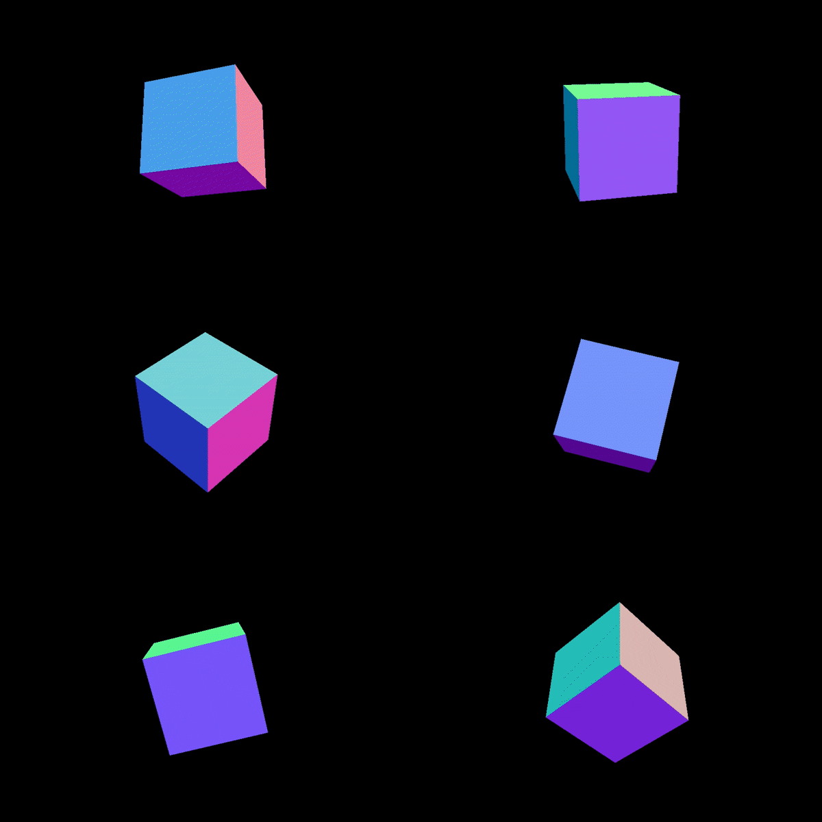
var material = new THREE.MeshNormalMaterial();

This material uses the normals of the surface to decide the local colour.

That's a much clearer rendering of a 3d object.

Carl then introduced the idea of manual controls to orient the object. We include another library from three.js called OrbitControls.js.

<script src="https://threejs.org/examples/js/controls/OrbitControls.js"></script>

In our javascript we add the controls linked to the camera:

var controls = new THREE.OrbitControls(camera);

We remove the cube rotation from the animate loop and instead set the orientation using these control library.

controls.update();

We can now control how we view the scene by effectively moving the camera.

Now let's use the power of code to create lots of objects.

Let's replace the code that creates a single material and cube with a loop that creates many, padding each to an initially empty list.

var boxes = [];
var numBoxes = 9;
for (let x = -numBoxes; x <= numBoxes; x++) {
  for (let y = -numBoxes; y <= numBoxes; y++) {
    var material = new THREE.MeshNormalMaterial( );
    var cube = new THREE.Mesh( geometry, material );
    cube.position.x = x * 1.1;
    cube.position.y = y * 1.1;
    boxes.push(cube);
    scene.add(cube);
  }
}

To keep each cube independent, each needs a new instance of a material. The loop counters x and y are used to set the location of each individual cube.

The following shows the array of boxes this loop creates.

Let's now modify these. Inside the animate function we can adjust the positions and rotations of each of these cubes individually.

// work through each box
for (var box of boxes) {
  
  var x = box.position.x;
  var y = box.position.y;
  
  box.position.z = Math.abs(x) + Math.abs(y);
  
}

Here we've pulled out the x and y position of each cube and used it to set the z position. The calculation uses the Manhattan distance, which results in an arrangement that looks like this:

That's pretty effective!

Carl demonstrated other kinds of manipulation such as offsetting each cube using wavy trigonometric functions.

A key idea he did introduce was the use of a pseudo-timer to calculate box positions. The pseudo-timer variable, which we can call step,  is created in the main javascript code.

var step = 0;

It is updated inside the animate loop, incrementing it by 0.0001 with each call to animate().

// work through each box
for (var box of boxes) {
  step += 0.0001;
  
  var x = box.position.x;
  var y = box.position.y;
  
  box.position.z = Math.sin(step + Math.sqrt(x*x + y*y));
  
}

Here we set the z position of each box using a sine function that depends on the distance of the box from the origin, and also the step pseudo-timer.

That's a rather pleasing effect! The key point is the use of the pseudo-timer to adjust the positions of the boxes in the animate loop.

You can explore the code on glitch:

• https://glitch.com/~algorithmicartmeetup

Carl proceeded to look at more advanced ideas such as setting colours dynamically, adding additional lighting, and also grouping objects so they could be rotated together, or even adjusting the vertices of each object. Do look through his tutorial to explore these ideas in more detail.

The group enjoyed Carl's tutorial and we reflected that his introduction took away most of the initial barriers to trying a new technology. Several said they'd go home and continue to explore three.js.

References

Friday, 22 February 2019