Thursday 13 June 2019

How Simple Maths Makes Beautiful Mandelbrot Fractals

This month's meetup in Cornwall aimed to demystify how the famous Mandelbrot and Julia fractals are created.

We were also lucky to have Brod Ross, an artist from Falmouth, who shared his work and process creating stunning 3d scenes based on fractal constructions.


The slides are online: pdf.


Organic Patterns

We started by taking a look at examples of patterns that looked organic and natural but were in fact created by a mathematical process.

Here is an example that has very fine filament-like details, combining a feeling of detailed thread work or the growth of an exotic plant.


The following is another example that looks like an underwater scene of seahorse-like creatures.


These patterns are entirely generated by a mathematical process. This surprises many as they're very organic and natural in form.

The previous two patterns are details from the famous Mandelbrot fractal. The following are examples of a related mathematical pattern called a Julia fractal.


These are more self-contained and a higher degree of symmetry.


These patterns are fractals - they are self-similar at different scales.

These fractals are named after the key characters who either discovered them, or did much of the ground-breaking work in the mathematical processes that create them - Benoit Mandelbrot and Gaston Julia.


Simple Maths

We then took our first gentle steps into mathematics to prepare ourselves for the ideas that lie behind these fractals.

The following expression x2 + c is rather simple. All it says is "square a number and add another number to it". Square means "multiply by itself".


For example, if x is 2 and c is 3, then x2+ c is 4 + 3 = 7.

Easy enough.

Yet surprisingly, this is the formula at the heart of the Mandelbrot and Julia fractals.

The stark contrast between the simplicity of this formula and the extremely detailed organic fractals we've seen is a perfect example of how mathematics has a beauty, hidden not too far under its surface!

Let's take another step.

The way this simple formula is used, is to take the answers it gives us and feed them back in again. The following picture explains this idea better.


So if x started at 2, and c is 3, we've seen the result is 7. Let's put that back in. So 72 + 3 = 52.

We can think of x2 + c as a machine that we feed, and that spits out an answer.

Let's look at a simpler example using a simpler machine:


This machine is simply x2. If we start feeding it 2, it spits out 4. If we feed that 4 back in again, it spits out 16. The sequence of numbers being spat out grows larger and larger through 256, 65536, and 4294967296 and upwards.

What happens if we start with not 2 but 0.5. The numbers seem to get smaller and smaller.

The starting number seems to decide whether the numbers get bigger or smaller.


Let's make a map of how numbers behave - a map showing whether numbers get bigger and bigger, or smaller and smaller.

The following shows the number 2 coloured green, because iterated through the x2 machine it gets bigger and bigger.


The next picture shows the number 0.5 coloured red, because iterated through the machine the numbers get smaller and smaller.


If we continue to test lots of numbers on the number line, including negative numbers we get a map that looks like this:


The negative numbers smaller than -1 are green because they do get bigger and bigger. Negative numbers squared become positive. The red region is around 0 and that makes sense because fractions less than 1 get smaller and smaller.

The map also shows 1 and -1 coloured blue because those numbers, when iterated through x2, don't get bigger or smaller, they stay at 1. The blue dots mark the boundary between the red and green territories.

So far, the maths has been easy. Let's take one more step.

Let's keep the idea of feeding a machine like we have before. Let's keep the idea of drawing a map to show how starting numbers behave.

But let's change the numbers to another kind of number called a complex number, even though they aren't complex at all!


Complex Numbers

Complex numbers aren't complex. They are just a composite number made of two normal numbers.


One part is called the real part, and the other is called the imaginary part. We mustn't let this surreal naming scare us away!

Things made of 2 parts or 2 numbers aren't unfamiliar. We're used to latitude and longitude on geographical maps, chess board positions or cells in a spreadsheet.


Because complex numbers have 2 parts, we can visualise them on a 2d surface like a grid or a map. It is normal for the real part to be along the horizontal direction, and the imaginary part along the vertical direction.

If we want to push these numbers through our machine, we need to know how to add and multiply them.

Adding complex numbers is easy - we just combine real parts with real parts, and imaginary parts with imaginary parts:


Multiplying is also simple in principle. We combine all the elements just like we might multiply out brackets at school algebra:


We can sweep together real parts and imaginary parts but we're left with an element with i2. In the above example it is 3i * 5i = 15i2.

What is i2? Let's look at the following picture showing what happens when 1 is multiplied by i. The result is a rotation of 90 degrees anticlockwise.


Another multiplication by i means another similar rotation which leads to -1.

So i2 = -1.

We can now finish our multiplication:


So now we know how to add and multiply complex numbers, we're ready to feed these numbers to a machine again.


We'll start x at 0 + 0i which is the complex number for 0. We can choose a complex number for c, we just need to stick with it consistently through all the calculations.

Because complex numbers are 2 dimensional, the map we draw to show how they behave as we iterate them through the x2 + c function will be 2 dimensional too.


Surprising Behaviour of Complex Numbers

Let's see what happens is we start with x = 0 + 0i and c = 2 + 2i.


We can see the complex numbers get bigger rand bigger. The second value is 2 + 2i, the third is 2 + 10i, and the fourth is -94 + 42i. On the graph we can see the numbers are spiralling outwards.

The following picture shows this spiralling out, and also the direct distance to the point - the magnitude of the complex number. We can see the magnitude gets bigger quickly.


Let's try c = 0.4 + 0.4i.


This time we can see the numbers spiralling around before finally escaping. The magnitude chart shows this eventual explosion. This is interesting behaviour given how simple the function x2 + c is.

Let's try c = -0.3 + 0.4i.


The numbers seem to be getting sucked into an orbit around a specific point, and getting sucked inwards to that point - like a black hole. That point, in mathematical terms, is called an attractor.

More interesting behaviour!

Let's try c = 0.3 + 0.5i.


This time the orbit is more sustained and has a larger shape. Another kind of behaviour - all from the innocent looking x2 + c.

What could a map of this behaviour look like?

The following shows an early plot created in 1978!


The map isn't a circle or a square, an oval or a diamond. It is a strange beetle shape!

Again - this strangeness from the innocent x2 + c function!

Here is a higher-resolution plot of the map, showing which numbers explode and which fall towards zero.


Finally ... the famous Mandelbrot Set.

We can see self-similarity in the pattern. There are smaller bulbs on the main bulbs, and each one of those has smaller bulbs too.

Let's remind ourselves how the image is created:


We pick a point on the 2-d map to test. We push that number as c through the function x2 + c, repeatedly feeding the answer back into the function. If the numbers get larger and larger we colour the point white. If the numbers fall towards zero, we colour them black.

We saw earlier that sometimes the numbers seem to orbit around a point, not exploding or diminishing. These are at the boundary of that beetle, dividing the two kinds of regions.

The most popular renditions of the Mandelbrot fractal are coloured. There are many options for choosing how to colour the fractal, but the following is a popular option:


We still colour black the regions that fall towards zero. For the regions that explode, we identify how fast the numbers grow and use this rate to choose a colour.


When calculating the numbers, we can stop if the magnitude get's larger than 2. There is a mathematical proof that shows that if a number get's larger than 2, then it will escape.


We also set a maximum for the number of times we iterate the function because we don't have all the time in the world to see if a point diverges or converges. If the size reaches 2 before this maximum is reached, we can use the actual iteration count as a measure of how fast the number escapes, which we can use for the colouring.

The fractal is infinitely detailed, and we can set the "window" size to see the detail more closely.


That simple zooming-in reveals an incredible amount of beautiful detail - all from that very simple function!

The following youtube video shows an animated zooming into the Mandelbrot fractal ... the level of detail is breathtaking!


You can find commented Python code to draw a Mandelbrot set here:


Julia Sets

The Julia fractals are created in an almost identical manner. There is only one change:


With the Mandelbrot fractal, we start z as 0 + 0i and c as the point being tested.

With the Julia fractal we set z to start as the point being tested, but set c to a constant all over the map.

In effect, the roles of z and c are swapped.

Here is another nice example of a Julia set.


Sample Python code for creating a Julia set is here:


3D Landscapes

We previously used the rate of escape to choose a colour. We can also use this rate as a height of a point on a 3d landscape.

Here is the simple Mandelbrot fractal transformed into a 3d landscape surface.


A closer zoom into a Julia fractal creates a more interesting landscape:


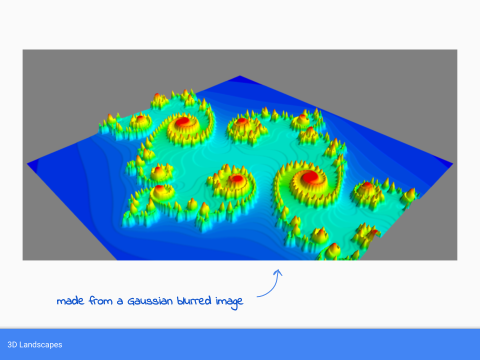
Being able to interactively move around and explorable a landscape is an interesting experience:


The code for creating and exploring landscapes like this is online too:


Mandelbulb Worlds

We were lucky to have Brod Ross show some of the worlds he creates using tools which create an almost photorealistic rendering of scenes containing objects that are fractals creates in basically the same way as the Mandelbrot and Julia sets.


Here are some of his works:


If you look closely, you can see the fractal nature of the structures.


Tools

If you want to use tools to explore these fractals, the following are good starting points:


Thursday 6 June 2019

Generative Adversarial Networks with PyTorch

This month's London meetup was an introduction to Generative Adversarial Networks, or GANs, currently a hot topic in machine learning and data mining.


The aim of the talk was to:
  • provide a beginner-friendly introductory overview of GANs
  • demystify how they work, avoiding unnecessary maths and jargon
  • explain the basic of PyTorch, a python machine learning framework
  • provide practical tutorial code to explore
  • share some of the current heuristics used to make GANs work

The slides for the talk are here: (pdf).

A video recording of the talk is here: (link).


Four-Part Blog

The journey of learning about GANS and writing simple examples is detailed in this 4-part series published on my other blog. This talk is the result of much of the learning and content created during that journey.
  • Part 1 introduces the idea of adversarial learning and starts to build the machinery of a GAN implementation.
  • Part 2 extends the code to learn a simple 1-dimensional pattern 1010.
  • Part 3 develops our code to learn to generate 2-dimensional grey-scale images that look like handwritten digits
  • Part 4 further develops our code to generate 2-dimensional full-colour images of faces, and also develops a GAN based on convolution layers to learn localised features.

I won't repeat the content of those blogs here - you should read those for a fuller yet gentle journey from preparatory basics through to a working convolutional GAN.

Here I'll set out the key steps taken in the talk.


GANs? Adversarial Learning?

We started by playing a game which challenges us to see if we can tell real photos from computer generated faces apart.


The computer generated images are surprisingly realistic and it was genuinely difficult to tell them apart. See for your self at http://www.whichfaceisreal.com/

These images are generated by GANs, and the game demonstrates their effectiveness.

We also talked about the growing interest in creating art with GANs. A key milestone in the history of art is the sale of a Portrait of Edmond Belamy at Christies for $432,500 in October 2018.


That portrait was generated entirely by computer, using a GAN.

Robbie Barrat, who created the code behind that portrait, himself has some stunning images created by GANs. This is one notable example:


Before diving into GANs, we refreshed our understanding of basic machine learning and how neural networks work.


In essence, neural networks are trained by feeding them data, images for example, and comparing their actual output to the known-good output. This difference, the error, is used to adjust the link weights inside the network with the aim of producing a slightly better output.

Neural networks can be trained to perform tasks like classifying images - and a common tutorial example is to learn to classify images of human handwritten digits, known as the MNIST dataset.

Make Your Own Neural Network is an accessible introduction to neural networks designed for beginners which starts from scratch and builds a simple neural network to classify these digits.


We proceeded to learn about PyTorch, a python framework which makes doing machine learning easier. In particular it provides automatic gradient calculation, which is a critical part of updating a neural network. Previously the algebra and calculus had to be done by hand, but today toolkits like PyTorch can do this automatically for many kinds of networks we might want to build.

A working notebook showing this capability was demonstrated, using Google's colab service:


PyTorch also makes using a GPU to accelerate machine learning very easy. Again a simple live notebook was demonstrated to show the key code elements:


Using the GPU does have some overhead which means for small tasks the benefit isn't there, but as the following graph shows, the benefits emerge as we scale the data or size of neural network we're training:


A simple example of PyTorch code to classify the MNIST images was explored.


Using this simple example, we focussed on the machinery of PyTorch code - subclassing from the nn.Module class, building up network layers, choosing a loss function and an optimiser for performing the network updates.


This code pattern will remain pretty much the same as our code grows, so is a good educational example.

We finally asked what a GAN was.

We started by looking at the architecture of simple machine learning. A machine learning model, which can be a neural network but doesn't have to be, has its internal parameters adjusted in response to the error it produces:


We then looked at the GAN architecture:


We have a learning model, a discriminator, which it is trained to separate real data from fake data. On its own that's just like a typical machine learning system. We also have a second machine learning model, a generator, which learns to generate data with the aim of getting it past the discriminator.

If this architecture works well, the discriminator and the generator compete to out-do each other.

As the discriminator gets better and better at telling real from fake data apart, the generator also gets better and better at generated fake data that can pass as real.

A common analogy is of a forger learning to get better at fooling a policeman or detective:


This adversarial dynamic is quite unique and in fact a relatively recent invention (Ian Goodfellow, 2014), and is the reason the architecture is called a generative adversarial network.

We then proceeded in steps to develop our GAN code. We started first with a simple example learning a 1-dimensional 1010 pattern:


The simplicity of the task allowed us to focus on the machinery again, especially the collection and display of the error, often called the loss.


Normally the loss is expected to fall to zero in a normal network, but with a GAN the discriminator should find it harder and harder to tell apart the real data from the generated data - and so the error should approach 1/2 (or 1/4 if we're using mean squared error as in the picture above).

The following shows visually how the output of the generator improves as training progresses. You can clearly see the 1010 pattern emerge.


The next step was to learn 2-dimensional data, images, and the monochrome MNIST dataset is ideal:


The shape and nature of the discriminator followed the simple classifier we developed earlier - a simple network with one middle layer. The input size is fixed at 784 because the images are 28x28. The output size is 10 to match the 10 digits.


The generator is often designed first as a mirror of the discriminator, and then adjusted as required.

The results looked disappointing:


The generator has failed to learn to draw digits, and all the images look very similar.

We discussed how, in general, GANs are hard to train, with common pitfalls like mode collapse where only one of many possible solutions is found by the generator.


It is worth remembering that a successful GAN is a fine equilibrium between the generator and the discriminator.

The next version of the code implemented some common improvements - using a leakyRELU activation instead of the vanilla sigmoid because it doesn't suffer from vanishing gradients, layer normalisation to rescale network signals to the sweet spot for the activation functions, and a stronger Adam optimiser which works per-learning parameter.


The results looked much better:


Those generated images are impressive if we remember that the generator has not seen the real images from the data set at all. We've also avoided mode collapse too.

We then moved beyond the monochrome images to full-colour photos of celebrity faces, using a popular CelebA dataset of 200,000 images. For our experiments, we used only 20,000.


The code itself didn't need any structural changes, only needed to adapt to the new 3-channel images and larger but still simple neural networks:


The results were impressive in that a diverse set of faces were indeed generated:


There are faces with different skin colour, different hair styles, and even different pose orientations too.

It is wort noting that the GAN approach doesn't learn "average faces". What is learned is a probability distribution from which samples can pass the discriminator. This is why the generated images are nicely diverse.

A second round, epoch, of training improves the images:


And more training improves the images again:


Much further training led to a degradation of image quality, which suggests we've reached the limits of our intentionally simple architecture.

The animated image at the top of this post shows several generated images being interpolated smoothly. They are generated by moving a consecutive sequence of 1's across the 100-long input array.

We next looked at convolutional neural networks. The reason for this is that convolution layers learn localised image features, and are well suited to image  classification tasks.

The following diagram shows how a convolution kernel pick out diagonal patterns in the source image and builds a feature map.


We can set a neural network to learn these kernels by itself instead of predefining them. Here is a simple example of an MNIST classifier that uses convolution layers:


For a GAN, we hope that a convolution layers in the generator will learn to build an image from features, perhaps elements like eyes, noses, lips etc.


At first the results from the generator were not as expected, reflecting the difficulty of designing and training a GAN:


That GAN was rather good at generating horror characters!

After some trial and error, a successful and still simple GAN was found:

  • https://github.com/makeyourownalgorithmicart/makeyourownalgorithmicart/blob/master/blog/generative-adversarial-network/04_celeba_gan_conv.ipynb


The results were impressive. The following from one training epoch shows how the faces are indeed being patched together from learned features.


A second epoch improves how the faces are constructed.


Six epochs again shows some improvement.


Eight epochs results in faces that are starting to be constructed more smoothy.


The following is an animation of several generated faces smoothly transitioned just for effect.


Although these images might not win awards for fidelity, they do show that even a very simple network using only a few lines of code can still create fascinating images.

They're fascinating because the generator has never seen the real images, and has still learned to construct faces from features it has also learned indirectly via the discriminator.


Conclusion

I was really pleased the talk matched the audience's expectations of an introductory talk that demystified GANs, and also provided simple tutorial code and summarised a few of the heuristics currently used to make them work.