We just had an interesting
meetup session introducing
ray-tracing, a method which aims to create realistic computer generated scenes.
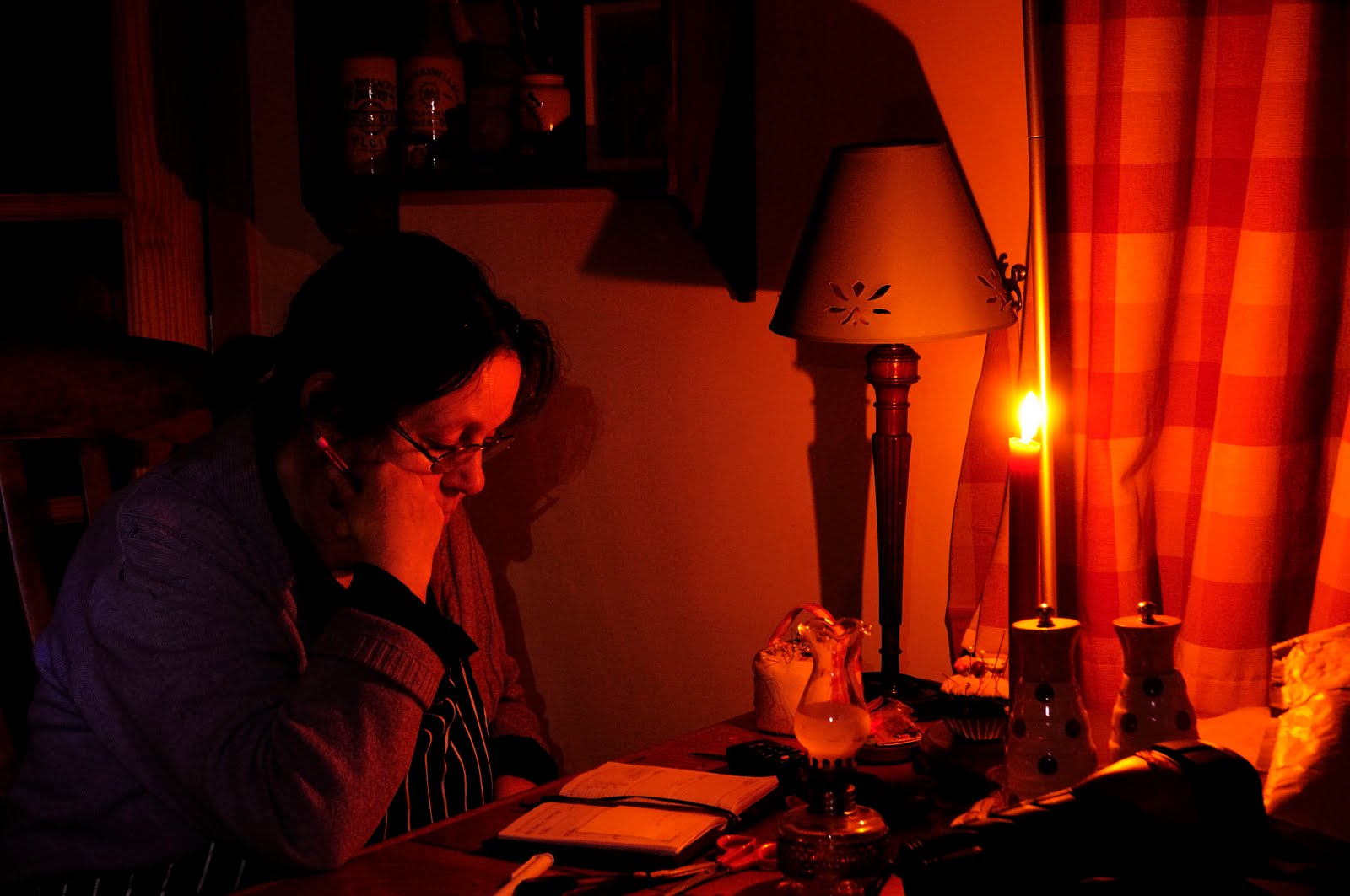
Here's an example of a ray-traced scene which is so realistic it's hard to believe that it was crafted only from mathematics. Nothing in this image exists in real life as a physical object for us to photograph.
Here are the
slides,
video, and example
code on GitHub.
The Challenge - Render a Realistic Scene
Ever since they were able to create coloured marks on a screen, we've set ourselves the challenge of getting computers to render scenes which are realistic. Scenes realistic enough to look like they had been filmed or photographed, rather than obviously looking like they had been generated by a computer program.
This is a great challenge for many reasons. Practically, we can save on the costs and effort of building physical objects and scenes. Creatively, we are free to imagine all kinds of objects, things, and make them appear real. That in itself, is a big enough reason to take up this challenge.
Over the last few decades, the sophistication of our image making methods has grown massively, helped by a similar exposition of computing power to makes these dreams feasible. Even today there is furious competitive activity trying new ideas to make computer generated scenes more realistic. And it's not just for stand along art, there is a huge hunger for better, more realistic, and more efficient rendering in the film effects and gaming.
The following image, amazingly, is not a photograph. It is entirely generated from a mathematical model of the pebbles. It was created a few years ago, using free open source
software. Leading visual effects companies will be using even more sophisticated tools today.
Ray-Tracing - Inspired by Physics
So, how do we render a scene, when the objects in the scene are only imagined? There are several approaches we could take. We could just use a painting program and lay down digital brush strokes, to build up an image, just like we would a traditional painting.
Another approach is to think about how nature itself lights a scene, and to try to replicate that in a computer program. That means we're thinking about how light starts at a light source, like the sun, and arrives at a scene, how it falls onto an object, and is perhaps reflected around the scene, or perhaps diffused or absorbed by some materials, before some of it finally enters our eyes for us to perceive the scene.
Trying to follow rays of light around a scene, which includes light sources, objects and ourselves as an observer, is called
ray-tracing.
Thought this tutorial we'll try to think about this challenge in plain English first. It's a great way of understanding ideas first, making sure they're sensible, way before attempting to encode them as mathematics or computer code.
Basic Elements of A Scene
Let's be clear about what elements make a scene. We've already said we have
objects in the scene - they're the things we're most interested in portraying. They might be balls, boxes, or more complex objects. We know we need light to be able to see anything. Without light, the scene would be pitch black. So we need a
light source, or maybe more than one.
It's tempting to stop there, but we need to also think about ourselves as an observer in the scene. What we see depends on where we're located, and the direction in which we're looking. If you're a photographer, you'll be very aware of this!
The following summarises these key elements.
We've included one more element in the scene, a
viewport. The idea is to take a rectangle out of around everything to frame a scene. You'll have seen film directors do the same.
It's a nice coincidence that the rectangular framed view is analogous to a computer display (like a laptop screen) and the rectangular format of computer image files.
Follow The Light
Ok - we now have a simple example scene - with the sun as a light source, a red sphere, and ourselves as observers. What next?
We know that we can only see the sphere because light falls on it. And that light must emerge from the light source. That all sounds obvious, but hang in there.. there's a reason for being so explicit about this.
So to simulate this working of nature, we need to draw rays of light from the light source and see where they land. The following shows some rays emerging from the sun.
You can see how some rays never really go anywhere near the sphere, and that's what we expect. Light from the sun shoots out in all directions. Some light does travel in the vicinity of the red sphere but just misses it, and carries on past our area of interest.
Some light rays do hit the sphere. Finally! Let's not get too excited just yet .. some of those rays of light do hit the ball but then bounce out of the scene away from our observing eye. That means those rays of light don't carry any information to our eyes about the scene. In some sense, they're useless to us for rendering the scene. There are some rays that, thankfully, do hit the ball and bounce straight into our eyes, carrying with them information about the colour of the ball.
Great! We've already found a way of building up a scene by following rays from a light source, and selecting only those that get bounced into our eyes. You can see why the technique is called
ray-tracing - because we're tracing rays of light through the scene.
That is an achievement - especially if you've never ever considered how to computationally render a scene before.
There is one problem with that initial (good) idea thought. It's extremely inefficient. If you think back to that light source, we know light shoots out in all directions. And the vast vast majority won't go anywhere near the objects of interest. And of the ones that do, a tiny fraction will make it through the viewport and into the observing eye. We'd be wasting so much computer calculations and time following rays which ended up elsewhere.
What's the answer? It's actually really simple and elegant. We work
backwards!
Backwards Ray-Tracing
We know we're only interested in light that ends up in the eye, so why not start there and work backwards. This is in fact most ray-tracers work - by tracing rays, from the observer, backwards through the scene. The following shows this:
That diagram also starts to hint at how we might choose rays to follow. You will know that computer images are made up of pixels, little squares of colour. Computer displays are made up of pixels, and computer image files (like jpegs, or pngs) contain information about the pixels in an image.
We need to know what the colour of every pixel in that rectangular frame should be. That means we need to cast a ray from the eye, through each pixel in the viewport. if we did any less, we'd have missing pixels in the computer image we're trying to render.
Next we need to think about how we actually work out whether a ray touches an object or not.
Rays Hitting Objects - Intersection
This section will get a little bit mathematical ... but we should always keep in mind what we're trying to do. In plain English - we're trying to test whether a ray hits an object or not. Simply that.
How do we even get started with this? Well - we need a mathematical way of describing both the ray and the spherical ball.
- The ray (straight line) is easy. It has a starting point, and a direction. Both can be described using vectors, which many will have learnt about at school. Vectors have a direction, not just a size, this is really useful for us when raytracing.
- The sphere (ball) is also easy. To define a sphere, we need to know where its centre is, and how big the sphere is .. which it's radius tell us neatly.
The following summarises how we define a ray and a sphere mathematically.
That's the basic idea but we need to be able to write these ideas in precise (mathematical) form.
A ray line is described by the starting point $\mathbf{C}$ and points along a direction $\mathbf{D}$. How far along that direction is controlled by a variable parameter, let's call it $t$:
$$ \mathbf{R} = \mathbf{C} + t \cdot \mathbf{D}$$
For small $t$ the point is close to the start, and for larger $t$ the point is further away along the ray.
A sphere is described by remembering that every point on its surface is always the same distance from the centre, that distance being the radius $r$. If they weren't the object might be a lumpy blob! For any point $\mathbf{P}$ on a sphere centred at $\mathbf{S}$ we have
$$ | \mathbf{P} - \mathbf{S} | = r $$
If we square both sides, the logic is the same, but the algebra is easier later:
$$ | \mathbf{P} - \mathbf{S} |^2 = r^2 $$
We've created mathematically precise descriptions of two objects - that's an achievement!
Now we need to work out whether the ray actually hits the sphere or not. This may not seem obvious, but the way to do this is to equate the two mathematical descriptions, and see what falls out of the algebra. By equating the two expressions, we're saying that a point is on the line
and it is also on the sphere. What should drop out is the point (or points) at which this is true. If the ray doesn't touch the sphere, the algebra should tell us somehow, perhaps by collapsing to an impossibility like $t^2 = -4$ which doesn't have any real solutions for $t$.
The following illustrates the equating of the line and sphere expressions, and the algebra that emerges. It looks complicated but it's just expanding out brackets which many will have done at school.
Expanding out the terms results in an
quadratic equation in $t$. Yes it looks complicated, but it is still a quadratic equation, the same that many solved at school. The general formula for solving quadratic equations $ax^2 + bx + c = 0$ is
$$ x = \frac{-b \pm \sqrt {b^2 - 4ac} } {2a} $$
We don't need to calculate the full solution for $t$ to know whether the ray touches the sphere. The reason is that if we look at the generic solution, there is a bit ${b^2 - 4ac}$ which tells us whether there are 2 solutions, 1 solution (2 repeating), or no real solutions .. remember that quadric equations have 2 solutions. Because that bit is so useful it is often called a
determinant, $\Delta$. For us, that determinant is
$$ \Delta = 4 \mathbf{D}^2 \cdot ( \mathbf{C} - \mathbf{S})^2 - 4 \mathbf{D}^2 \cdot ( \mathbf{C}^2 + \mathbf{S}^2 - r^2) $$
The following shows what it means for this determinant to be more than, less than or equal to zero:
It's nice to see that a quadric equation emerges, and that it has 2 solutions .. because a ray can intersect a sphere at 2 points. And it's nice that the maths neatly captures the scenario when the ray misses the sphere.
Ok - enough of the maths symbols. Back to ray tracing. Our test for whether the ray touches the ball is simply $\Delta >= 0$. That's it!
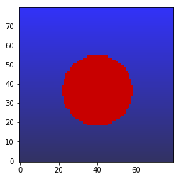
Let's try it .. the results are:
Our very first ray traced scene! That's a big first step. We've managed to describe a scene mathematically, with a light source, an observer, a viewport, and an object .. and we've used the mathematical descriptions to follow rays back from our eye to see if they hit the sphere. You can find example Python code to do all this on
github.
Take a well-deserved break before we continue.
Shading
That sphere we rendered above is great, but it doesn't look three dimensional. The thing that gives the impression of three dimensions, of solidity, is how light is different at different points on an object.
Let's think about a real sphere .. like a snooker ball. There will be light and dark bits. The light bits are the ones that are facing the light source most directly. And the dark bits are the ones that are pointing away from the light source. The following diagram shows this.
We've described that in plain English and it makes sense. How do we translate that idea into maths?
Luckily the answer is easy. We can consider the angle between the normal at each point of the sphere and a vector to the light source. A normal is just a vector pointing directly out from a surface, so it meets the surface at right angles. The following shows these angles:
The small the angle, the more more directly that bit of surface is being illuminated. The larger the angle, the less directly.
Maths is kind to us here. The cosine function nicely indicates this alignment, with the cosine of smaller angles being closer to one, and as the angle grows, the cosine gets smaller ... and negative once the vectors point away from each other. Even better, we don't need to calculate the cosine of the angle, or even the angle itself, because a simple dot product of the two vectors indicates the same quantity because $\mathbf{a} \cdot \mathbf{b} = ab \cdot cos(\theta)$. We just need to make sure we normalise the dot product so that longer vectors don't bias it.
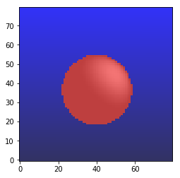
Let's try colouring the pixels according to how aligned the intersected points on the sphere are to the light source. The result is ...
Much better .. It's starting to look three dimensional and solid.
This simple approach to shading a surface, based on how directly it is illuminated - is good enough for many applications. But we want to develop the realism further.
The next improvement is to realise that what we've done is to only consider how well a point on an object is illuminated. That's not the same as considering how much light is reflected to the observer's eye. The two things are distinct but related. First a surface is illuminated by a light source, then some of that light is reflected away, perhaps towards the observer, but mostly likely not.
The following diagram shows why only considering illumination is not enough. The two points shown have the same illumination, but one reflects light to the observer more directly than the other, which actually reflects it away.
We can reuse our idea of using angles to see how directly any reflected light travels to the observer. A small angle means the light is reflected more directly into our eye.
How do we work out what the reflected ray is? This diagram explains best the link between the vector from a point on the surface to the light source, $\mathbf{L}$, and the reflected ray, $\mathbf{R}$.
The two rays $\mathbf{L}$ and $\mathbf{R}$ are like mirror reflections about the normal $\mathbf{N}$. If we add them together we should get a result that's straight up the normal, but perhaps a different length. That symmetry is what will help us work out $\mathbf{R}$.
$$ \mathbf{L} + \mathbf{R} = 2 (\mathbf{L} \cdot \mathbf{N}) \mathbf{N} $$
That's just saying the sum is twice the projection of \mathbf{L} onto \mathbf{N}. It's super easy to re-arrange to
$$ \mathbf{R} = 2 (\mathbf{L} \cdot \mathbf{N}) \mathbf{N} - \mathbf{L} $$
The following shows the two effects we're taking into account now - illumination and reflection to the observer.
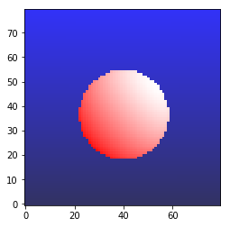
Combining these two effects to modify the base red colour of the sphere gives us the following result.
That's much much more realistic. We can see a highlighted area of the surface, and a darker area too, which is just like real spheres that we see.
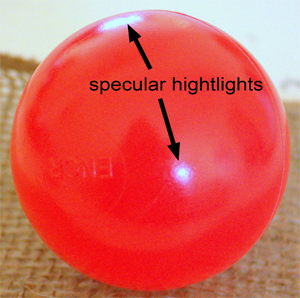
Phong Specular Highlights and Matt Surfaces
We considered how we might model the specular highlights, often seen in more shiny or glossy surfaces. This photograph of a snooker ball shows these high-intensity highlights clearly, and we recognise them as characteristic of smooth, glossy shiny objects.
A simple approach is to squeeze the function that maps the angle between the normal and the light source. That way, the increase in light is focussed on a smaller bit of the surface. That worked but actually the light intensity wasn't increased, so the highlight area just became smaller. A lesson learned there is to increase the intensity of the contributed light as that function is squeezed. This squeezing is called
Phong highlighting.
The opposite of shiny, glossy is to a matt surface that diffuses light that falls on it. If we think about how light is reflected from such a surface, we realise that the surface is very irregular at a small scale, and this causes light to bounce in all sorts of random directions, including into nooks and crannies so that it never emerges. The following illustrates this.
How do we describe this behaviour in mathematics. There are several ways, including randomising the normal so the reflected ray is bounced in different directions. Another approach is to keep the normal as it is, but add a small random vector to the reflected ray. That's a milder adjustment but does seem to work, as the following comparison between a shiny and a matt ball shows.
The example code is on
github.
Reflections
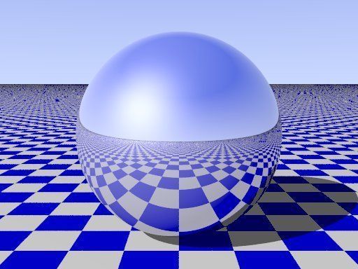
Being able to show realistic reflections is one of the key things that attract people to ray-tracing. Everything we've done up to this point can be approximated well enough without the very involved calculations required by ray-tracing.
In the 19080s ray-traced images like the following were state of the art, used to show off the cleverness of the software creator and the power of computers.
How do we include reflections into our ray-tracer?
Let's think again in plain English before we dive into any maths. We already have the idea of a reflected ray worked out and being used. A reflection is simply us being another object on the surface of an object we're looking it. That means the light has bounced from another object onto the one we're looking directly at, before arriving at our eyes. The following image shows this more clearly.
Following rays backwards, you can see that one of the paths taken by the ray (shown in orange) hits the first object, is reflected into a second object and then a third object before it finally goes back to the light source.
We have some new thinking to do here .. so take a break, a coffee or a breath before proceeding!
Reflection Depth
How many reflections do we want to model? This is a good questions because reflections could go on forever, and we don't want to get stuck in a computational rabbit-hole!
We don't want to write a program that is specific to a number of reflections. We want a program where the
depth, or number, of reflections is configurable.
A good way to do this is to make the ray a
recursive function. A recursive function is one that calls itself. That might be a bit mind boggling, but have a look around the internet for simple
examples.
The reason this powerful idea suits ray-tracing reflections is that each ray creates a new ray when it hits an object, that is, the reflected ray .. and that ray in turn can create another reflected ray when that hits an object .. and so on .. until we reach a depth at which we want to stop.
The following diagram shows the ray function spawning another ray function ... and it also shows what information is passed back up the chain - the colour information at each object ... which we want to accumulate. This is right because when we see reflections we're looking at the accumulation of colour information from all subsequent reflections.
To make a recursive function work, we need to think really carefully about what information it takes as input, and what information it accumulates and returns. For us, this isn't so difficult. A ray function needs to know
- the start position of the ray,
- the direction, and
- the current depth
and it returns
- whether the ray intersected an object or not
- the accumulated colour (which may have been added to on intersection)
You can see from the diagram that for a maximum depth of 3, it is possible for a ray to have collected information from 3 onward reflections and intersections.
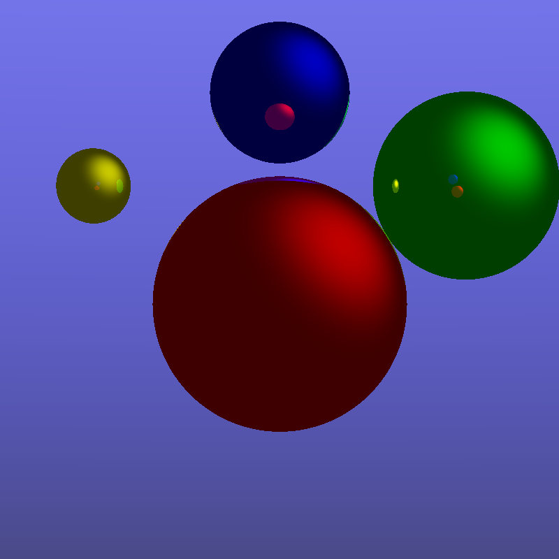
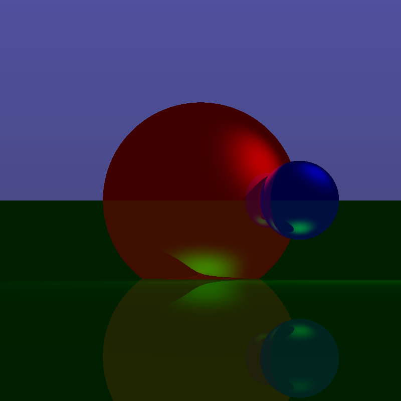
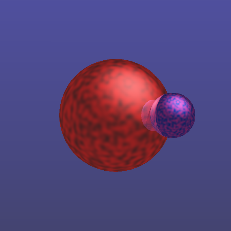
Let's see some results:
That's pretty amazing! We can see the green ball reflected in the yellow ball. In fact we can also see the red ball reflected in that yellow ball too.
We have reflections working! Example code is at
github.
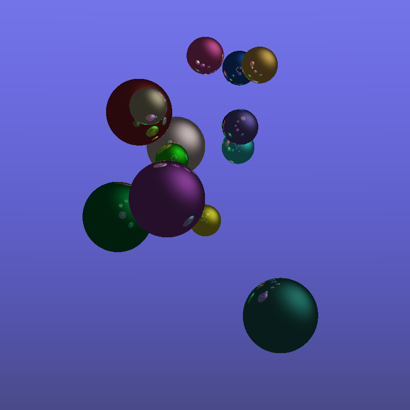
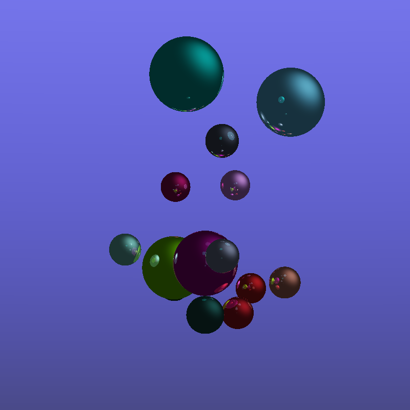
Random Spheres Art
Here's a nice triptych of random spheres, with reflections a key feature. It's created using only the ideas we've worked through above.
Objects in Ray-Tracing
Before we go on to define another kind of object, in addition to the sphere we have worked with up to now, it is worth thinking about the minimum set of things any such object definition must provide.
There are only 3 things:
- being able to test whether a ray intersects the object or not
- being able to provide a normal vector (pointing out) at any point on the object
- a material colour at any point
Any kind of objects, simple like a plane, or complicated like a torus, must be able to provide those three bits of information when needed. Let's look at a plane next.
Flat Plane
How do we define a flat plane mathematically? It may not be obvious but it is true that we only need a point on the plane and its normal vector. That is, a point, any point, through which the plane lies. This pins it to a point in space. But the plane could have any orientation through that point, which is why we need the normal to tell us which way the plane is facing. The following diagram illustrates this.
We now need to work out how to test for intersection. That's actually easy, because a ray will always hit an infinite flat plane unless it is parallel to it. But we need to know where a ray hits a plane, so that we can then work out things like reflections and illumination from a light source.
The key to this is to realise that a vector from that defining point, let's call it $\mathbf{X}$, and a point $\mathbf{P}$ on that plane, is always perpendicular to the normal, $\mathbf{N}$. The following illustrates this:
Let's write out what we just said, in mathematical form:
$$ (\mathbf{P} - \mathbf{X}) \cdot \mathbf{N}= 0 $$
Substituting that point $\mathbf{P}$ with the definition of a ray,
$$ (\mathbf{C} + t \cdot \mathbf{D} - \mathbf{X}) \cdot \mathbf{N}= 0 $$
It's really simple to re-arrange that so we have $t$ on one side:
$$ t = \frac{(\mathbf{X} - \mathbf{C}) \cdot \mathbf{N}} {\mathbf{D} \cdot \mathbf{N}} $$
That bottom part of the fraction, $\mathbf{D} \cdot \mathbf{N}$, like a determinant we saw before. If it is zero, we can't divide by zero, and so there is no intersection. That's when $\mathbf{D}$ and $\mathbf{N}$ are perpendicular (ray parallel to plane).
The results do work well ... but only after we refine the accumulation of colour by diminishing how much is accumulated in proportion to the depth - otherwise an unrealistic amount of light is accumulated as the number of reflections increases. See the slides for more detail on this.
Texture
In real life, most objects aren't uniformly coloured. They have variations of colour in, often recognisable, patterns. Wood and marble stone patterns are easily recognisable, for example.
How do we add texture to our objects. At the moment we're using a simple base colour, like red for the sphere we started with. We know we need to vary the colour that's returned when a ray intersects an object .. but how do we vary it?
We know a pattern is spatial - the variation in colour depends on the location we're looking at. This is the key. We need to be able to connect, link a location on an object with a part of a known pattern. As we vary the location on the object, we move around the pattern. We can do this in two ways - we can have a pattern that is a bitmap image texture, or we can use a mathematical expression to define a pattern.
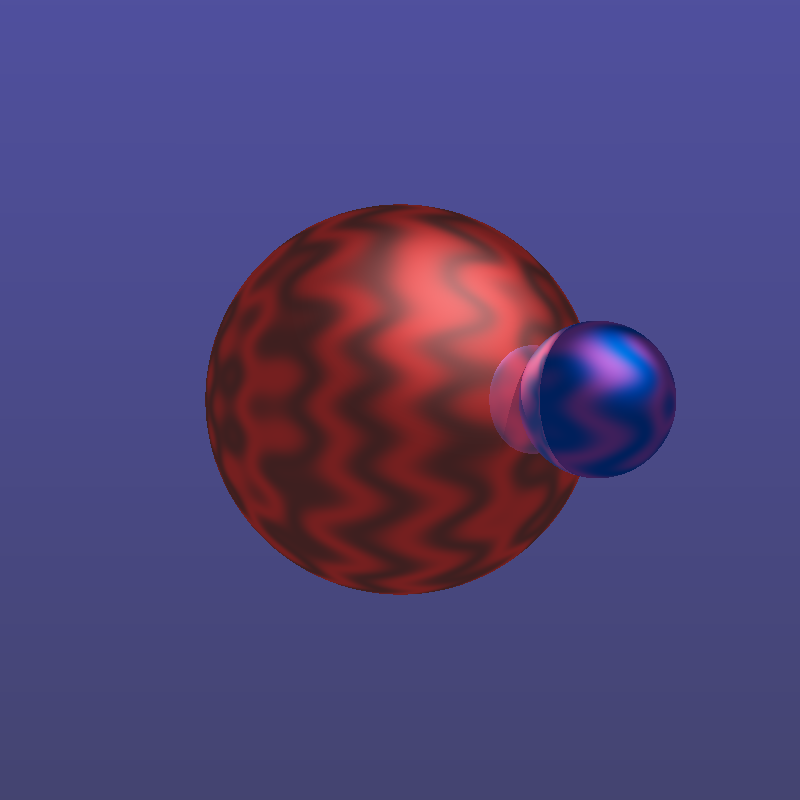
Here's an example of a texture defined by a mathematical expression where the red element of the objects colour is $sin(3x) + sin(4y) + sin(4z)$.
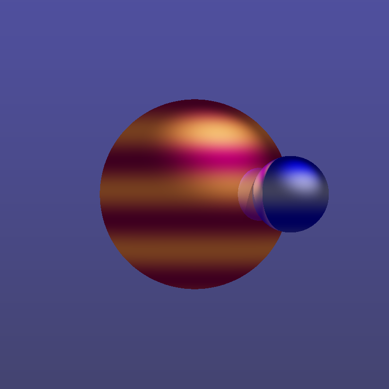
Here's one where the colour is defined only by the vertical $y$ component of the position, where the red element is $sin(y^2)$.
Here's one where the texture is defined by a bitmap of a marble texture.
The reason the texture looks oddly stretched is because it is not trivial to map a flat texture to a spherical surface .. the same problem as projecting the Earth's surface to a flat map.
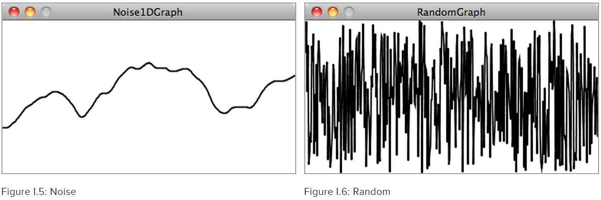
We can even use a function for random noise to define a texture. Purely random noise isn't always useful in many areas of computer graphics. Instead, a smoother noise is more realistic. Often Perlin noise, or
OpenSimplex noise, is used .. you can see from this comparison the difference. With this kind of noise, successive values are close to previous values, making the transition similar to real world phenomena like mountains or clouds.
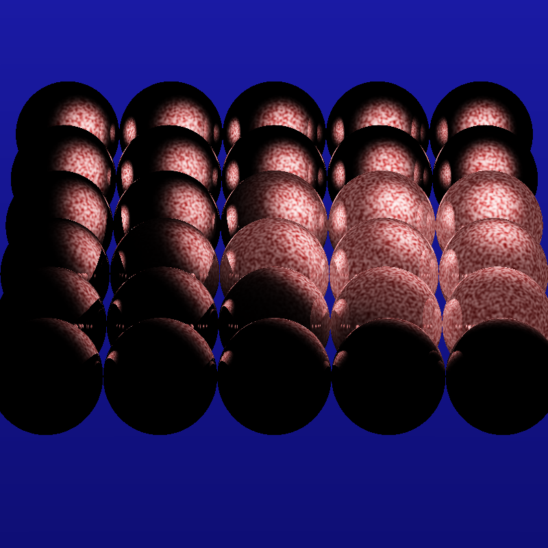
The following shows sphere textures based on opensimplex noise using the $(x,y,z)$ components of the surface normal.
These are really nice, and because we use the surface normal, we avoid the problems of mapping spherical surfaces to 2-dimensional textures.
Mathematically defined textures are really fun to experiment with, and the possibilities are endless!
Light-Fall Off
A nice lighting effect which we see in photography and in paintings is light falling very rapidly with distance from the light source.
This should be easy to implement. We simply need to calculate the distance from an intersection point to the light source and apply a function which forces a rapid fall off.
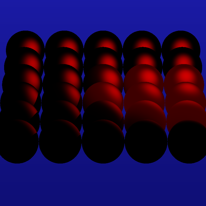
In physics, we know the light should fall off as an inverse square of the distance. In practice, we can use sharper functions to exaggerate the fall-off for artistic effect. Here's an set of functions based on $tanh(x)$.
The effect is rather pleasing:
Using the effect on textured objects also works well:
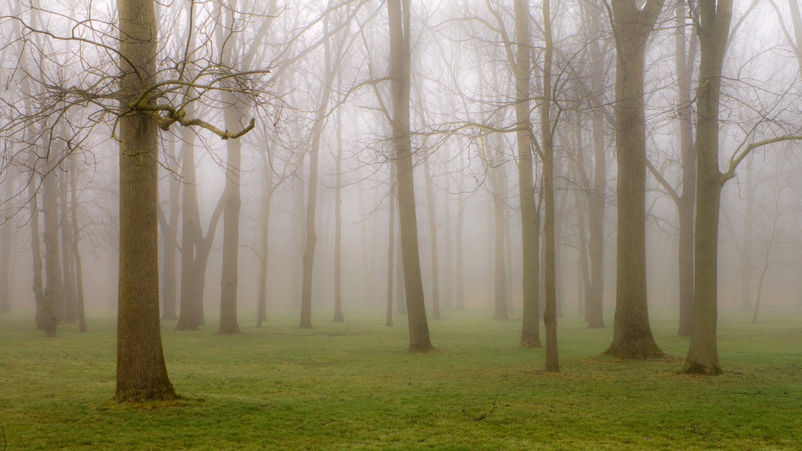
Fog
The last effect we looked at was fog. This is different to everything we've looked at before because it is an atmospheric effect, not an effect on the surface of objects.
There are many methods for modelling atmospheric effects, and we'll look at two simple ones.
The first is one inspired by how many textbooks describe atmospheric effects. They think of a fog as a volume, through which light passes, and has a chance of interacting. This makes sense. Fog is made of particles (just as smoke is), and light can pass through it, or hit a particle, which is why fogs obscure a scene.
The deeper the fog, the larger the probability that a light ray has hit a fog particle. For rays that don't hit an object, but carry on out of the scene, we can set an artificial large distance. The results look like this:
Well, we do see a diminishing of colour for distant objects, but the overall effect isn't very pleasing. The image is too grainy, and the background is unrealistic.
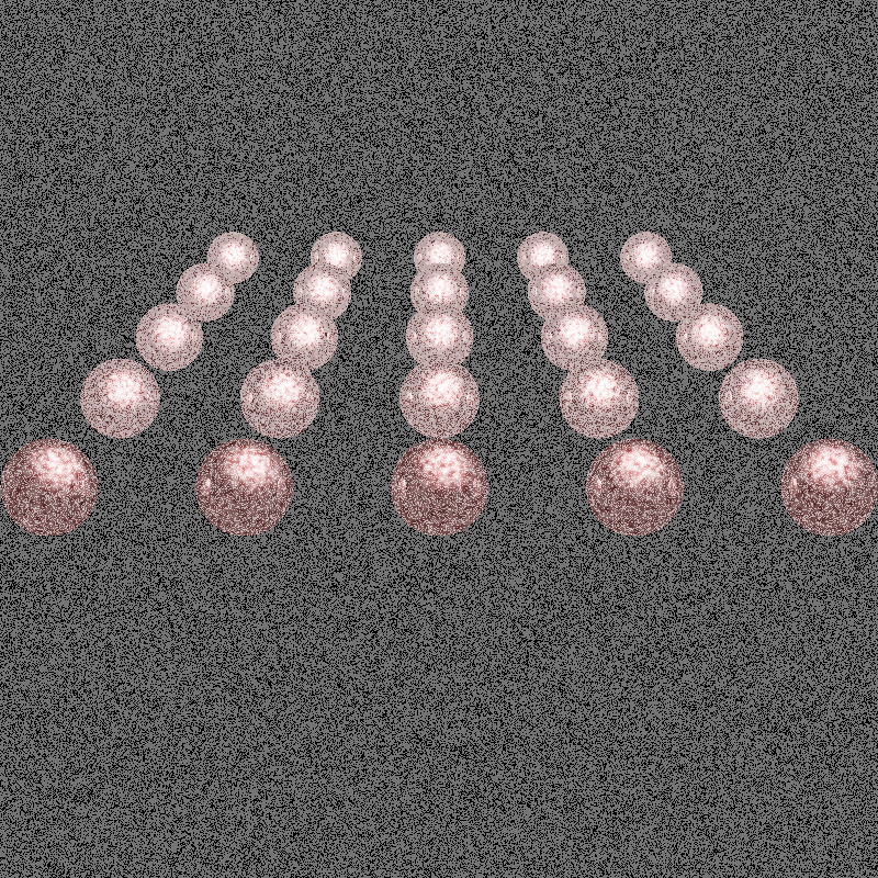
Let's try again, and think in plain English for ourselves. We want to have a smoother diminishing of object colour with distance, towards a fog colour (white, but could be black or brown smog). We can try using a smooth gradient and not the speckling effect we get from the random probability method above. We also want to have some variation in our fog, a lumpy fog. We can use a noise function to create this. Here's a summary of the idea:
For testing we'll use a more visible green fog, to see more clearly the effects of our ideas. Here's an image of just the lumpy noise applied:
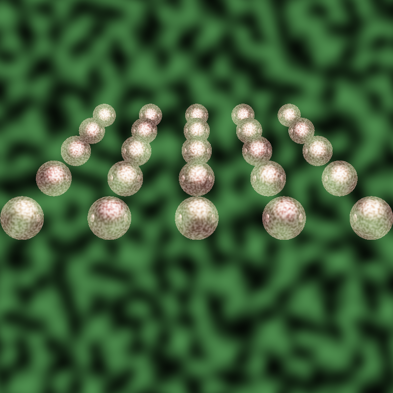
Here's the result with the lumpy fog texture augmented with the distance based intensity.
Looking at one of the closer spheres, you can indeed see the lumpiness of the fog.
POV-Ray
Finally, we looked at a real ray-tracer. There are several expensive and very sophisticated software renderers, some very proprietary to visual effects companies, we looked at
POV-Ray.
POV-Ray is free and open source, and was started around 1986. It was very popular in the 1990s and early 2000s as being the leading, and accessible, ray-tracing software. I myself spent many hours exploring POV-Ray, using a book, before the internet was as rich and available as it is now.
I would encourage you took explore POV-Ray because you describe a scene in simple code, and this forces you to understand more closely the effects and methods being applied.
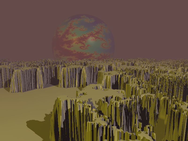
Here's a simple scene created in POV-Ray:
The foreground is a height field created from an image of a
Julia fractal. The sphere moon ha a texture where the colours are also based on the same fractal image.
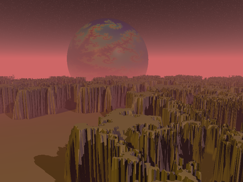
We can add fog to the image to create a more realistic image:
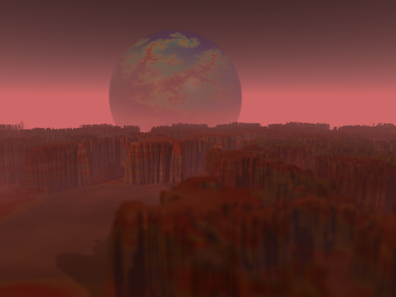
We can improve this even further by applying a focal plane effect where objects nearer or further from that plane are blurred, much like a real camera with a large aperture. The landscape has also had a texture applied to it too, giving it the appearance of stratified rocks.
Not a bad result for such a short time experimenting with POV-Ray!
All the code is available on
github.
Interesting Questions
There were some great interesting questions from members of the audience during and after the meetup:
Q. Real objects absorb and reflect certain parts of the light spectrum. How does this ray-tracer reflect that?
A. It doesn't. Our simple ray-tracer has a very simple model of light, reflection and accumulating object colour. Today's most sophisticated ray-tracers do model light as a continuum of frequencies and more correctly model the selective absorption of certain frequencies by different materials.
Q. Accumulating colour with larger depths can cause the values to overshoot the normal colour range (0-255 for RGB values). How do you handle this?
A. You're right and the slides do show this overshoot happening. I switched from integers (uint8) to floating point (float64) numbers for the colour components. This way I don't need to worry about overshooting. Before the image is rendered, a squishing function based on $tanh()$ again is used to bring all tlevalues back into the 0-255 range. This also has the benefit of handling high and over saturation realistically.
Q. How long does it take?
A. Ray-tracing has traditionally been seen as very time consuming. This is still true today. Our own very simple code only takes seconds for moderately sizes images. The largest factor affecting ray-tracing time is the number of objects or the number of rays being spawned. A scene with 80 objects would take many minutes. Most of the simple scenes took a few seconds. This is very fast compared to computing in the 1980s which could take many hours or days. Our own code is in Python, a friendly easy to learn language, but not one that is very fast. POV-Ray is written in C/C++ and ism much faster, with single-sphere scenes being rendered almost instantaneously.
Q. Why don't you spawn multiple rays at each intersection, rather than just one?
A. That's a great idea for further exploration :)